3.7. Subplots

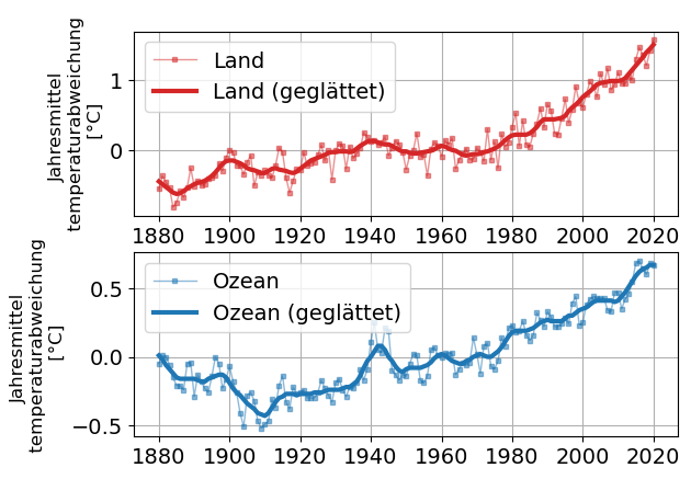
Mit Subplots können mehrere Plots in sogenannten axes innerhalb eines figures dargestellt werden

import matplotlib.pyplot as plt
import pandas as pd

# read data

link = "https://data.giss.nasa.gov/gistemp/graphs_v4/graph_data/Temperature_Anomalies_over_Land_and_over_Ocean/graph.csv"
Temp_NASA2 = pd.read_csv(link, header=1) # einlesen

# plot

plt.style.use('default')
plt.figure(figsize=(10,4))
plt.rcParams['font.size'] = 14;

fig, (ax1,ax2) =plt.subplots(2,1)

ax1.plot(Temp_NASA2["Year"],Temp_NASA2["Land_Annual"], ls="-", lw=1, marker="s", ms=3, color="tab:red", alpha=0.5, label="Land");
ax1.plot(Temp_NASA2["Year"],Temp_NASA2["Lowess(5)"], lw=3,  color="tab:red", label="Land (geglättet)");
ax1.set_ylabel("Jahresmittel \n temperaturabweichung \n [°C]", fontsize=12)
ax1.grid();
ax1.legend();

ax2.plot(Temp_NASA2["Year"],Temp_NASA2["Ocean_Annual"], ls="-", lw=1, marker="s", ms=3, color="tab:blue", alpha=0.5, label="Ozean");
ax2.plot(Temp_NASA2["Year"],Temp_NASA2["Lowess(5).1"], lw=3,  color="tab:blue", label="Ozean (geglättet)");
ax2.set_ylabel("Jahresmittel \n temperaturabweichung \n [°C]", fontsize=12)
ax2.grid();
ax2.legend();

<Figure size 1000x400 with 0 Axes>

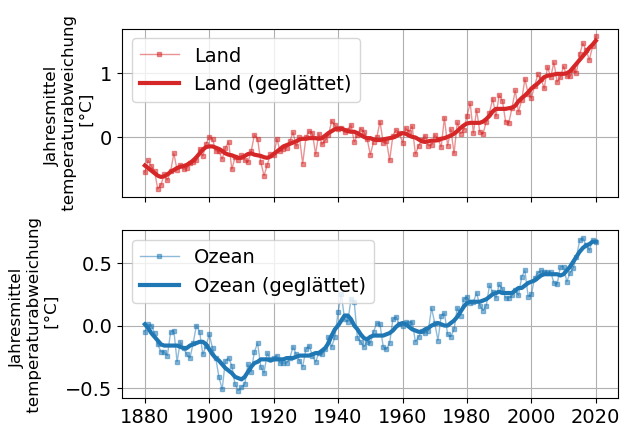
mit sharex=True kann z.B. die x-Achse für beide Plots verwendet werden

import matplotlib.pyplot as plt
import pandas as pd

# read data

link = "https://data.giss.nasa.gov/gistemp/graphs_v4/graph_data/Temperature_Anomalies_over_Land_and_over_Ocean/graph.csv"
Temp_NASA2 = pd.read_csv(link, header=1) # einlesen

# plot

plt.style.use('default')
plt.figure(figsize=(10,4))
plt.rcParams['font.size'] = 14;

fig, (ax1,ax2) =plt.subplots(2,1, sharex=True)

ax1.plot(Temp_NASA2["Year"],Temp_NASA2["Land_Annual"], ls="-", lw=1, marker="s", ms=3, color="tab:red", alpha=0.5, label="Land");
ax1.plot(Temp_NASA2["Year"],Temp_NASA2["Lowess(5)"], lw=3,  color="tab:red", label="Land (geglättet)");
ax1.set_ylabel("Jahresmittel \n temperaturabweichung \n [°C]", fontsize=12)
ax1.grid();
ax1.legend();

ax2.plot(Temp_NASA2["Year"],Temp_NASA2["Ocean_Annual"], ls="-", lw=1, marker="s", ms=3, color="tab:blue", alpha=0.5, label="Ozean");
ax2.plot(Temp_NASA2["Year"],Temp_NASA2["Lowess(5).1"], lw=3,  color="tab:blue", label="Ozean (geglättet)");
ax2.set_ylabel("Jahresmittel \n temperaturabweichung \n [°C]", fontsize=12)
ax2.grid();
ax2.legend(); 

<Figure size 1000x400 with 0 Axes>

3.7.1. Aufgabe

Plotten Sie die Jahres Temperaturabweichung (NASA Daten) und die CO2 Konzentration übereinander