1. Grundlagen¶

1.1. Daten¶

Daten eintragen¶

Als Python-Liste

keine Rechenoperationen möglich

x = [0,1,2,3,4]
y = [2,4,1,5,3]
y2 = [4,2,5,1,0]

Als numpy-Array

import numpy as np
x = np.array([0,1,2,3,4])
y = np.array([2,4,1,5,3])
y2 = np.array([4,2,5,1,0])

Als pandas-dataframe

Die Werte für x werden dann mit df["x"] abgerufen

import pandas as pd

df = pd.DataFrame({'x':[0,1,2,3,4], 'y1':[2,4,1,5,3], 'y2':[4,2,5,1,0]})

Daten von Datei einlesen¶

ToDo hier muss noch Inhalt rein ...

Funktionen¶

ToDo hier muss noch Inhalt rein ...

1.2. Import der Matplotlib Bibliothek¶

import matplotlib.pyplot as plt

1.3. Scatter/Linien Plot¶

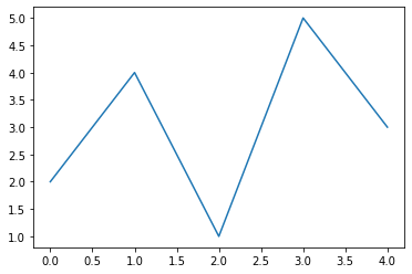
Tipp: Das Komma nach dem letzten Befehl hat nur einen kosmetischen Grund, weil es die Ausgabe des letzten Befehls unterdrückt.

plt.plot(x,y);

Linien (Typ , Farbe , Dicke)¶

Hinweis zur Linienfarbe: Wenn die Linienfarbe selbstständig definiert wird, so wird für jeden neuen plot selbstständig eine neue Liniefarbe gewählt

ls - Linienstil

c - Linienfarbe

lw - Liniendicke default=1

Bilder aus: offizielle CheatSheets von Nicolas P. Rougier

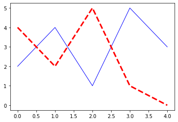
plt.plot(x,y,ls="-",c="blue",lw=1);
plt.plot(x,y2,ls="--",c="red",lw=3);

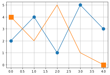
Marker (Typ , Farbe , Dicke)¶

marker - Markerstil

markevery - Anzahl

ms - Markergröße

Bilder aus: offizielle CheatSheets von Nicolas P. Rougier

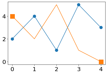
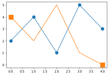
plt.plot(x,y,marker="o",ms=10);
plt.plot(x,y2,marker="s",ms=15,markevery=[0,-1]);

1.4. Beschriftungen¶

Achsenbeschriftung¶

plt.xlabel(" ")
plt.ylabel(" ")

bzw.

ax.set_xlabel(" ")
ax.set_ylabel(" ")

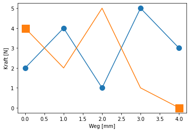
plt.plot(x,y,marker="o",ms=10);
plt.plot(x,y2,marker="s",ms=15,markevery=[0,-1]);
plt.xlabel("Weg [mm]");
plt.ylabel("Kraft [N]");

Bildüberschrift¶

plt.title(" ")

bzw.

ax.set_title(" ")

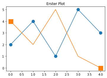
plt.plot(x,y,marker="o",ms=10);
plt.plot(x,y2,marker="s",ms=15,markevery=[0,-1]);
plt.title("Erster Plot");

Legende¶

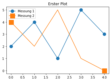
label=' ' Bennenung im plot Befehl
plt.legend() Legende anzeigen

ToDo Legenden Positionen

plt.plot(x,y,marker="o",ms=10, label='Messung 1');
plt.plot(x,y2,marker="s",ms=15,markevery=[0,-1], label='Messung 2');
plt.title("Erster Plot");
plt.legend();

1.5. Wertebereich der Achsen¶

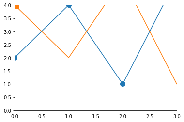
beide Werte vorgeben:

plt.xlim(x1,x2)
plt.ylim(y1,y2)

nur einen Wert vorgeben:

plt.xlim(left=x1) oder plt.xlim(right=x2)
plt.ylim(bottom=y1) oder plt.xlim(top=y2)

plt.plot(x,y,marker="o",ms=10);
plt.plot(x,y2,marker="s",ms=15,markevery=[0,-1]);
plt.xlim(0,3);
plt.ylim(0,4);

1.6. Gitter¶

plt.grid()

plt.plot(x,y,marker="o",ms=10);
plt.plot(x,y2,marker="s",ms=15,markevery=[0,-1]);
plt.grid();

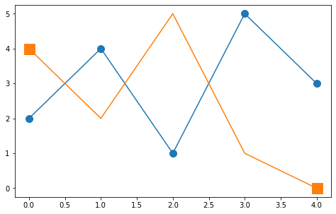
1.7. Bildgröße¶

Hinweis: Befehl muss vor dem plotten kommen

plt.figure(figsize=(8,5)) - Größe in inces (Default: 6,4)

plt.figure(figsize=(8,5));
plt.plot(x,y,marker="o",ms=10);
plt.plot(x,y2,marker="s",ms=15,markevery=[0,-1]);

1.8. Schriftgröße¶

Hinweis: globaler Paramter bleibt für alle weitern Plots aktiv können aber mit ( mpl.rcParams.update(mpl.rcParamsDefault ) zurückgesetzt werden.

global:

plt.rcParams.update({'font.size': 20})

individuell:

ToDo

plt.rcParams.update({'font.size': 20});
plt.plot(x,y,marker="o",ms=10);
plt.plot(x,y2,marker="s",ms=15,markevery=[0,-1]);

1.9. Bild speichern¶

plt.savefig('Name.png', bbox_inches='tight', dpi=150)

plt.plot(x,y,marker="o",ms=10);
plt.plot(x,y2,marker="s",ms=15,markevery=[0,-1]);
plt.savefig('Name.png', bbox_inches='tight', dpi=150)